Gauss Quadrature Rules

1. Big Picture
2. Jacobi Matrix
3. Constant c
4. Open Source Code
Reference

This note is served as a summarization of Gauss quadrature rules. There are lots of theoretical results either in the textbooks or papers. The main focus of this note, however, is to implement it with actual code from scratch. I will also try to provide some theoretical background when necessary and provide the sources where the readers can find the proofs.

1. Big Picture

In this section, I will set up a toy problem and the process to tackle it with Gauss quadrature rules. In the later sections, I will try to introduce more applications.

Goal: Our target is to estimate

$\int_{-1}^{1} f(x) dx,$

using numerical approximations (assume that the function is ‘nice’).

We all know how to do this with Riemann sum:

$\int_{-1}^{1} f(x) dx \approx \sum_{i=1}^{n} f(x_i^*)(x_{i+1}- x_i), \tag*{}$

where $-1=x_0\leq x_1 \leq \cdots \leq x_n = 1$ is a partition of the interval [-1,1], $x_i^*$’s nodes selected in between $x_i$ and $x_{i+1}$. Gauss Quadrature rules aim to do the same thing. It tries to do the approximation in the following way:

$\int_{-1}^{1} f(x) dx = \sum_{i=1}^{n}w_i g (x_i) + R[f], \tag{Gauss Quadrature}$

where $g(x)$ will be a modified version of $f(x)$ according to the ONP, $R[f]$ is the residual of the approximation which depends on the regularity of $f(x)$. Of course, no matter what kind of approximations we do, the errors should always depend on both the approximation rules and $f(x)$ itself. The art part of Gauss quadrature rules is to find the $w_i$ (called weight) and $x_i$ (called node) such that $R[f]$ is as small as possible.

To make this part short, I will list several key facts of Gauss Quadrature rules. Later on I will try to provide some proofs.

Key Fact:

Gauss Quadrature rules are indeed a class of rules. Each of them is associated with a choice of orthonormal polynomials (ONPs). For example, Gauss quadrature rule with Legendre polynomials, Gauss quadrature rule with Chebyshev polynomials of first kind, etc.
The nodes $x_i$ of a specific Gauss Quadrature rule are selected as either zeros or the local extrema of the associated ONPs.
Every ONP satisfies a three-term-recurrence-relation (3TRR), which will implicit indicate that the ONP can be defined through a special tridiagonal matrix $J$ called Jacobi matrix.
Given a specific ONP, the eigenvalues of the Jacobi matrix $J$ are the zeros of it. In other words, it gives the nodes $x_i$.
$J$ is symmetric and has eigenvalue decomposition $J = Q\Lambda Q^T$. The weights $w_i = c q_{1i}^2$, here $q_{1i}$ is the $(1,i)$th entry of matrix Q and $c$ is a constant depends on the ONP that is used.

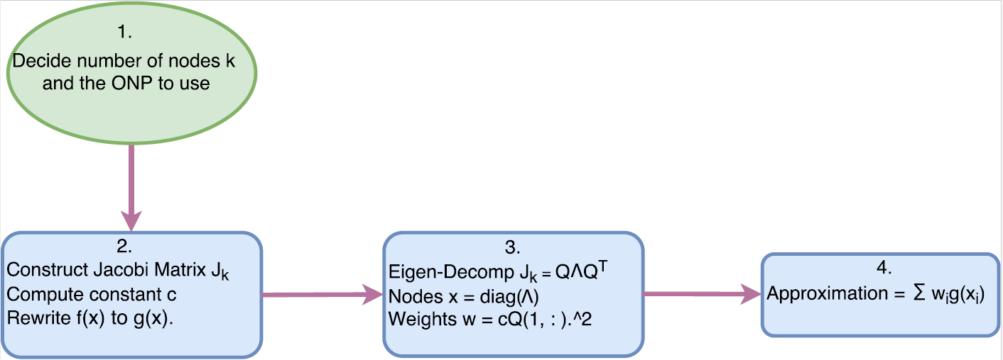
Now we summarize the whole procedure of using Gauss Quadrature rules to approximate the integral.

Workflow:

Example time!

A simple example is to calculate the Gauss Quadrature rule with Legendre polynomials. I will list some basic facts and we will discuss in details later.

Facts of Legendre polynomials:

The Jacobi matrix of Legendre polynomial is

$J_k = \left( \begin{array}{ccccc} 0 & \beta_1 & & & \\ \beta_1 & 0 & \beta_2 & & \\ & \beta_2 & 0 & \ddots & \\ & & \ddots & 0 & \beta_{k-1} \\ & & & \beta_{k-1} & 0 \end{array} \right)$

Here $\beta_i = \frac{1}{2\sqrt{1-(2i)^{-2}}}$. Remember that it should be a tridiagonal matrix. $k$ is number of nodes.

The constant c for Legendre polynomial is 2.
The function $g(x)$ is the same as $f(x)$.

A simple Matlab code demo for Gauss Quadrature rule with Legendre polynomials, see reference [1]:

function I = Quadrature_Legendre(f,n)
% n-pt Gauss quadrature of f (with Legendre polynomials)

%============== 1. Construct Jk ====================
beta = .5./sqrt(1-(2*(1:n-1)).^(-2)); % 3-term recurrence coeffs
J = diag(beta,1) + diag(beta,-1); % Jacobi matrix

% ============= 2. Eigenvalue decomposition ========
[V,D] = eig(J);  
x = diag(D); [x,i] = sort(x); % nodes (= Legendre points)
w = 2*V(1,i).^2; % weights here constant c = 2.

%============== 3. Calculate the approximation.=====
I = w*f(x); % the integral from -1 to 1.

For example, to estimate $\int_{-1}^{1} x^{10} dx$ (where the true value should be 2/11), we use 6 nodes and Legendre polynomials. The Matlab code is as follows:

f = @(x) x.^10;
n = 6;
I = Quadrature_Legendre(f,n);

The output is

I =  
>> 1.818181818181822e-01

The absolute error

abs(I - 2/11)
>> 3.885780586188048e-16

2. Jacobi Matrix

From the previous section, you know that the first step and also a crucial step is to figure what the Jacobi matrix is, given a specific ONP. The short answer is, for some well known ONP, such as Chebyshev polynomials (both first kind and second kind), Legendre polynomials, Laguerre polynomials, the Jacobi matrix is known.

Before my next step, let us ask a question:

Q: What exactly does it mean for polynomials to be orthogonal?

A: The inner product is 0.

We now define the inner product of polynomials. Given polynomials $p(\lambda)$ and $q(\lambda)$, the inner product (with respect to) the measure $d\alpha(\lambda)$ is defined as

$<p,q> = \int_{a}^{b} p(\lambda)q(\lambda) d\alpha(\lambda).$

For classical ONPs, the measure $d\alpha(\lambda)$ is known as well.

The following theorem may be helpful to understand where the Jacobi matrix comes from.

Theorem 1 (3TRR): For ONPs, there exists sequences of coefficients $\alpha_k$ and $\beta_k$, $k = 1,2,…$ such that (three-term-recurrence-relation)

$\beta_{k+1} p_{k+1}(\lambda) = (\lambda-\alpha_{k+1})p_k(\lambda) - \beta_kp_{k-1}(\lambda), \hspace{0.2in} k = 0,1,2...$

$p_{-1}(\lambda) \equiv 0, \hspace{0.2in} p_0(\lambda) \equiv 1/\beta_0, \hspace{0.2in} \beta_0^2 = \int_{a}^{b} d\alpha(\lambda)$

where

$\alpha_{k+1} = <\lambda p_k, p_k>, \hspace{0.2in} \beta_{k+1} = \frac{\|p_{k+1}\|_\alpha^2}{\|p_k\|_\alpha^2}$

and

$\|p_k\|_\alpha = \bigg(\int_{a}^{b} p_k(\lambda)^2 d \alpha(\lambda) \bigg)^{\frac{1}{2}}.$

What this theorem indicates is that the ONPs can be expressed through two sequences of numbers $(\alpha_k)$ and $(\beta_k)$ ! Suppose now I know $p_k(\lambda)$ and $p_{k-1}(\lambda)$, this theorem says, if I know two more numbers $\alpha_{k+1}$ and $\beta_k$, I will know exactly what the next polynomial should be!

The Jacobi matrix of size $n \times n$ is defined by these numbers:

$J_n = \left( \begin{array}{ccccc} \alpha_1 & \beta_1 & & & \\ \beta_1 & \alpha_2 & \beta_2 & & \\ & \beta_2 & \alpha_3 & \ddots & \\ & & \ddots & \alpha_{n-1} & \beta_{n-1} \\ & & & \beta_{n-1} & \alpha_n \end{array} \right) .$

Furthermore, the Jacobi matrix $J_k$ satisfies

$\lambda \textbf{P}_k(\lambda) = J_k \textbf{P}(\lambda), \hspace{0.2in} \text{where } \textbf{P}_k(\lambda) = \left[\begin{array}{c} p_0(\lambda) \\ p_1(\lambda) \\ \vdots \\ p_{k-1}(\lambda) \end{array} \right].$

Remark*: in many cases, the coefficients in 3TRR will help us build a matrix. However, this matrix may not necessarily be symmetric (which is required for Jacobi matrix). We then need to symmetrize the matrix. I will show this in the following examples.

Examples of 3TRR and the corresponding Jacobi matrix:

`1. Chebyshev polynomial of first kind.

$C_{k+1}(\lambda) = 2\lambda C_k(\lambda) - C_{k-1}(\lambda)$ $C_0(\lambda) = 1, \hspace{0.2in} C_1(\lambda) = \lambda$

The associated measure $d \alpha(\lambda) = (1-\lambda^2)^{-1/2} d\lambda$.

The zeros of this polynomial has closed form

$\lambda_j = \cos(\frac{(2j-1)\pi}{2k}), \hspace{0.2in} j = 1,2,...,k.$

We have,

$\lambda \left( \begin{array}{c} C_0(\lambda) \\ C_1(\lambda) \\ \vdots \\ C_{k-2}(\lambda) \\ C_{k-1}(\lambda) \end{array} \right) =\left(\begin{array}{ccccc} 0 & 1 & & & \\ 1/2 & 0 & 1/2 & & \\ & 1/2 & 0 & \ddots & \\ & & \ddots & \ddots & 1/2 \\ & & & 1/2 & 0 \end{array} \right) \left( \begin{array}{c} C_0(\lambda) \\ C_1(\lambda) \\ \vdots \\ C_{k-2}(\lambda) \\ C_{k-1}(\lambda) \end{array} \right)$

For simplicity, I will write this as

$\lambda \textbf{C}_k(\lambda) = T_k \textbf{C}_k(\lambda)$

As you can see, $T_k$ is not symmetric. Never mind, we can apply a similarity transformation such that the Jacobi matrix $J_k$ will be obtained by

$J_k = D^{-1}T_k D$

Proposition 1: Given a tridiagonal matrix

$T_k = \left( \begin{array}{ccccc} \alpha_1 & w_1 & & & \\ \beta_1 & \alpha_2 & w_2 & & \\ & \beta_2 & w_3 & \ddots & \\ & & \ddots & \alpha_{k-1} & w_{k-1} \\ & & & \beta_{k-1} & \alpha_k \end{array} \right) .$

If $w_i \neq 0$ and $w_i\beta_i>0$ for $i = 1,2,…,k-1$, then $T_k$ can be symmetrized by $D^{-1} T_k D$, where

$D = \left( \begin{array}{cccc} \delta_1 & & & \\ & \delta_2 & & \\ & & \ddots & \\ & & & \delta_k \end{array} \right) , \hspace{0.2in}\text{where } \delta_1 = 1, \hspace{0.1in} \delta_j^2 = \frac{w_{j-1}w_{j-2}\cdots w_1}{\beta_{j-1}\beta_{j-2}\cdots \beta_1}, \hspace{0.1in} j = 2,3,...,k-1.$

The following code will symmetrize $T_k$ and thus obtain the Jacobi matrix

function [J, D] = symmetrize_T(T)
%-------------------------------------
% Symmetrize a tri-diagnoal matrix
% J = D^{-1}TD, D is a diagonal matrix
%-------------------------------------
a = diag(T);
w = diag(T,1);
b = diag(T,-1);
d = zeros(size(a));

% Calculate the diagonal entries of D
d(2:end) = cumprod(b)./cumprod(w);
d(2:end) = sqrt(d(2:end));
d(1) = 1;
D = diag(d);
Dinv = diag(1./d);

% Calculate the symmetric Jacobi matrix
J = Dinv*T*D;

`2. Chebyshev polynomial of second kind.

$C_{k+1}(\lambda) = 2\lambda C_k(\lambda) - C_{k-1}(\lambda)$ $C_0(\lambda) = 1, \hspace{0.2in} C_1(\lambda) = 2\lambda$

The associated measure $d \alpha(\lambda) = (1-\lambda^2)^{1/2} d\lambda$.

The zeros of this polynomial has closed form

$\lambda_j = \cos(\frac{k\pi}{n+1}), \hspace{0.2in} j = 1,2,...,k.$

We have,

$\lambda \left( \begin{array}{c} C_0(\lambda) \\ C_1(\lambda) \\ \vdots \\ C_{k-2}(\lambda) \\ C_{k-1}(\lambda) \end{array} \right) =\left(\begin{array}{ccccc} 0 & 1/2 & & & \\ 1/2 & 0 & 1/2 & & \\ & 1/2 & 0 & \ddots & \\ & & \ddots & \ddots & 1/2 \\ & & & 1/2 & 0 \end{array} \right) \left( \begin{array}{c} C_0(\lambda) \\ C_1(\lambda) \\ \vdots \\ C_{k-2}(\lambda) \\ C_{k-1}(\lambda) \end{array} \right)$

In this case, the matrix is symmetric. Therefore this matrix is $J_k$.

`3. Legendre polynomials.

$(k+1) P_{k+1}(\lambda) = (2k+1)\lambda P_k(\lambda) -kP_{k-1}(\lambda)$ $P_0(\lambda) = 1, \hspace{0.2in} P_1(\lambda) = \lambda.$

The associated measure $d \alpha(\lambda) = d\lambda$.

Furthermore, we have $\lambda \left( \begin{array}{c} P_0(\lambda) \\ P_1(\lambda) \\ \vdots \\ P_{k-2}(\lambda) \\ P_{k-1}(\lambda) \end{array} \right) =\left(\begin{array}{ccccc} 0 & 1 & & & \\ 1/3 & 0 & 2/3 & & \\ & 2/5 & 0 & \ddots & \\ & & \ddots & \ddots & (k-1)/(2k-3) \\ & & & (k-1)/(2k-1) & 0 \end{array} \right) \left( \begin{array}{c} P_0(\lambda) \\ P_1(\lambda) \\ \vdots \\ P_{k-2}(\lambda) \\ P_{k-1}(\lambda) \end{array} \right)$

Again, we have to symmetrize this matrix with the code mentioned before.

3. Constant c

Another question is to compute the constant c.

Indeed, the constant c can be obtained by

$c = \int_{-1}^{1} d\alpha(\lambda).$

For example,

`1. Chebyshev polynomial of first kind.

$c = \int_{-1}^{1} d\alpha(\lambda) = \int_{-1}^{1}(1-\lambda^2)^{-1/2} d\lambda= \pi.$

`2. Chebyshev polynomial of second kind.

$c = \int_{-1}^{1} d\alpha(\lambda) = \int_{-1}^{1}(1-\lambda^2)^{1/2}d\lambda = \frac{\pi}{2}.$

`3. Legendre polynomial.

$c = \int_{-1}^{1} d\alpha(\lambda) = \int_{-1}^{1}1 d\lambda = 2.$

4. Open Source Code

Indeed, there many variants of Gauss quadrature methods. Basically they assume some of the nodes are prescribed (pre-fixed).

The following MATLAB code provides Gauss quadrature rules with different polynomials and Gauss-Radau (1 pre-fixed node), Gauss-Lobatto (2 pre-fixed nodes) methods. It is designed mainly for demonstration of the ideas of Gauss Quadrature rules. Use it at your own risk.

The code can be found here.

Reference

[1] Lloyd N. Trefethen, Is Gauss Quadrature Better than Clenshaw–Curtis?.

[2] Golub & Welsch, Calculation of Gauss Quadrature Rules.

[3] Golub & Meurant, Matrices, Moments and Quadrature with Applications.