This is my notes on SIAM Imaging Conference, May 23, 8:15 am talk: Non-conformist image processing with graph Laplacian operators, by Peyman Milanfar, Google Research
The video talk and the slides can be found here.
Global vs. Local filters
Usually, we represent the filtering in the following way:
where y is a vectorized image, W is a data-dependent matrix, it can represent local filters or global filters:
- Local filter: Sparse, but high-rank
- Global filter: Dense, but low-rank
Q: Remember if W just represent a kernel such as Gaussian, [-1,1], it will not be data dependent, how can we get a data dependent kernel then?
1 Laplacian Operators
In imaging:
- (Anisotropic) Diffusion
- Curvature flow
- Adaptive sharpening
- De-blurring
- …
A Laplacian operation is just filtering/centered average:
Quick explanation of some terms:
- Conformity: uniform, homogeneous
- Gradient (Dirichlet) Energy:
1.1 Discrete (Graph) Laplacian
Given a point $z_i$, the Laplacian transform applies on $z_i$ is defined as:
Notice that, this is just a local average with certain weights . Usually, the depends on the Gaussian distance of and .
- Gaussian distance (Gaussian kernel) applied to the pixel value
according to the author, this is called photometric Gaussian Kernel. Another is Spatial Gaussian Kernel (applied to the physical location of the ith pixel):
Now
It’s called bilateral kernel.
Also notice that
(maybe unrelated, but same formula importance sampling technique in Bayesian?) Anyway, it says the unbiased estimate of $z_i$ will just be an expectation based on the weights.
I haven’t checked the proofs but intuitively it’s not hard to imagine that with more and more samples (denser and denser grids), the discrete Laplacian will converge to the continuous one (Ref: Lafon ‘04’, Belkin et al ‘05’, Hein et al ‘05’, Singer ‘06’).
Q: Wait, we know the matrix now, but where is (the Laplacian matrix)?
Laplacian matrix $L$ is defined exactly as in graph theory:
First, we define the degree of a vertex (pixel),
then the graph Laplacian is then
. Here we consider K is not normalized, otherwise the sum of the weights will be 1. Hence we get the definition $L = I - K$, which can be found in most of the graph theory textbooks.
In pure matrix perspective, the graph Laplacian has many interesting properties, the following is a table illustrate the many definitions of graph Laplacian and their properties:
| Graph Laplacian | Symmetric | DC eigenvector | Spectral Range | Reference |
|---|---|---|---|---|
| $L = D - K$ | Yes | Yes | [0, n] | Un-normalized Laplacian |
| $I - D^{-1/2} K D^{-1/2}$ | Yes | No | [0, 2] | Normalized, Chung ‘97’ |
| $I - D^{-1}K$ | No | Yes | [0, 1] | Random Walk Laplacian |
| $I - C^{-1/2}KC^{-1/2}$ | Yes | Yes | [0, 1] | ‘Sinkhorn’ Laplacian, M. ‘13’ |
A naive version of normalized Laplacian is And the corresponding filter $W$ is defined as $W = I - L = I - \alpha (D - K)$.
It’s kind of confusing if you think about the regular graphs where each vertex has the same degree, the above definition of $W$ gives back of $K$! You may also wonder why we need $W$ here, indeed, suppose you are interested in minimizing the discrete Dirichlet energy $|z^TLz$ (it’s not hard to show that this is the discrete version of the Dirichlet energy I mentioned before), then by gradient descent you will contour the update
Therefore, given a Laplacian matrix and an initial state of the image $z_0$, to minimize the Dirichlet energy, we just need to calculate $W$ first, and iterative update $z_k$ by $z_{k+1} = Wz_k$.
BTW, the Laplacian matrix is positive semi-definite, so the above target function is non-negative. There are many ways to prove this, one quick way is that $L$ by definition is diagonal dominant. The following theorems help me a lot and turn out to be very useful in many situations:
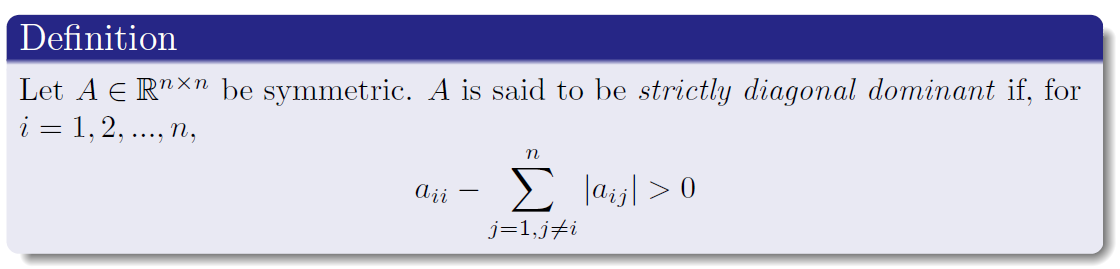
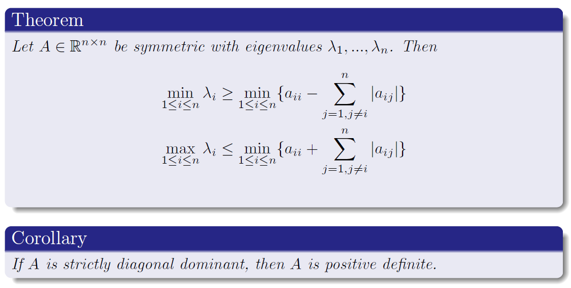
It can be shown that a Hermitian diagonally dominant matrix $A$ with real non-negative diagonal entries is positive semidefinite.
2 Application in Image Processing
2.1 De-blurring: adaptive sharpening
We can use the following model to do de-blurring, given blur matrix $A$:
Usually, I’d like to write the fidelity as . Basically, the difference between traditional norm and matrix is that may indicate correlation/covariance/weighted balance of the residual. It’s more flexible.
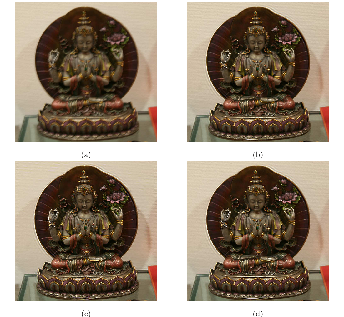
Most of the time we don’t have the knowledge of PSF (Point spread function), then we may simply solve the above optimization problem with , . Then the solution will be , for some ( a hand tunning parameter). This is called adaptive sharpening “nonlinear unsharp mask”.
The following image is cropped from
Motion De-blurring With Graph Laplacian Regularization, Kheradmand & Milanfar, 2015.
The code is here.
Let’s stop talking:
Here is some Matlab code on de-blurring with Laplacian from a NIPS paper:
Fast Image Deconvolution using Hyper-Laplacian Priors, Krishnan & Fergus, NIPS, 2009.
Code is here.
I will also write some code and will upload it later in github.
2.2 Linear Embedding Using Laplacian
I guess the this is the most interesting part of this post: Laplacian for manifold and hierarchical decomposition.
- Dimension Reduction
- Nystrom Approximation
- Multi-Laplacian Scale Decomposition
2.2.1 Dimension Reduction (DR)
A serious question before any fancy technique, what is dimension reduction? Think it again not just intuitively but also try to write some math definitions.
Recall the way we use PCA to do DR, we do the eigen-decomposition and then take the largest n eigenvalues and corresponding eigenvectors to approximate the original data matrix. Here the idea is the same, but little tricky.
We think the data points formulate the vertices of a ‘large’ graph.
The Laplacian DR algorithm basically goes with three steps:
- Given data points $x_1, x_2,…,x_k \in R^l$, build the graph: connect ‘near’ points with edges.
- Calculate the ‘Gaussian’ distance matrix W along the edges:
- Solve the following optimization problem:
This will reduce to a generalized eigenvalue problem:
where $D_{ii} = \sum_{j} W{ji}$, $L = D - W$, $L, D, W\in R^{k \times k}$.
Suppose we solved the optimization problem and get the eigenvector $y_0, y_1, …, y_{k-1}$, corresponding eigenvalues are $0 = \lambda_0 \leq \lambda_1 \leq \lambda_2 \leq … \leq \lambda_{k-1}$.
We can simply take the first few (say $m$) eigenvectors starting from $y_1$, and use them to ‘describe’ the original data:
Just as we pick up the first few PCA components! Because these contains the key information!
We will discuss it further in the next post.