Notes on LBFGS

Big Picture
Be Practical
Finally, the whole algorithm

This notes is from appendix of ‘Patch Ordering as a Regularization for Inverse Problems in Image Processing’ by Gregory Vaksman etc. and is part of the book ‘numerical optimization’ by J. Wright.

Another very nice reference: OverView of Quasi-Newton Methods.

L-BFGS is a limited memory quasi-Newton method, which approximates the inverse of the Hssian matrix instead of calculating the exact one. In additional, it stores only m vectors of length n (m « n) that capture curvature information from recent iterations, instead of saving the full n × n approximation of the Hessian.

Formulation

Let $f(x)$ be a smooth function with $x \in R^n$ .

Recall general Newton-method,

$p_k = -H_k^{-1}\nabla f(x_k), \\ x_{k+1} = x_k + \alpha_k p_k,$

k = 0,1,2…

The classical BFGS update is the following:

$H_+ = H_c + \frac{y_cy_c^T}{y_c^Ts_c} - \frac{H_cs_cs_c^TH_c}{s_c^TH_cs_c},$

where $H_c$ is current approximated Hessian, $y_c = \nabla f(x_+)-\nabla f(x_c)$ , $s_c = x_+ - x_c$ .

Big Picture

To be concrete, here is the whole framework:

Given $x_0$ , $H_0$ and $\nabla f(x_0)$
Update x: $x_{k+1} = x_k - H_{k}^{-1} \nabla f(x_k)$ ,
Update step: $s_{k} = x_{k+1}-x_k$ ,
Update gradient step: $y_k = \nabla f(x_{k+1}) - \nabla f(x_k)$ ,
Update Hessian: $H_{k+1} = H_k + \frac{y_ky_k^T}{y_k^Ts_k} - \frac{H_ks_ks_k^TH_k}{s_k^TH_ks_k}$

Be Practical

Well in practice, we don’t care about $H_k$ , instead we would like to calculate $H_k^{-1}$ directly according to the well known Sherman-Morrison-Woodbury formula. One can verify that the inverse Hessian has the scary update:

$H_{k+1}^{-1} = V_k^TH_{k}^{-1}V_k + \rho_k s_ks_k^T$

where $\rho_k = \frac{1}{y_k^Ts_k}$ , $V_k = I - \rho_k y_ks_k^T$ , $s_k = x_{k+1}-x_k$ and $y_k = \nabla f(x_{k+1}) - \nabla f(x_k)$ .

Notice: In textbook ‘numerical optimization’, $H_k$ denotes inverse of Hessian.

How can this help us?

Manually set a number m, we can recursively update $H_k^{-1}$ in the following way:

$\begin{aligned} H_{k}^{-1} &= (V_{k-1}^T...V_{k-m}^T)H_{k-m}^{-1}(V_{k-m}...V_{k-1}) \\ &+ \rho_{k-m}(V_{k-1}^T...V_{k-m+1}^T)s_{k-m}s_{k-m}^T(V_{k-m+1}...V_{k-1}) \\ &+ \rho_{k-m+1}(V_{k-1}^T...V_{k-m+2}^T)s_{k-m+1}s_{k-m+1}^T(V_{k-m+2}...V_{k-1}) \\ &+ ... \\ &+ \rho_{k-1}s_{k-1}s_{k-1}^T. \end{aligned}$

Ok now, let’s look at the formula above. If you are familiar with QR factorization in a recursive manner, don’t they look similar? You just recursively apply a linear operator $V$ on to initial $H$ and $s$ .

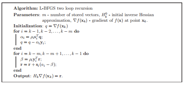
One step forward, the practical L-BFGS calculate $H^{-1}\nabla f(x)$ in its iterations. Here is the recursive algorithm:

Issue: before the second loop, should initialize $r = H_k^{-0}q$ . ( I use the notation $H_{k}^{-0}$ and to remind that they are the inversion of Hessian.) Also pay attention that the $H$ here is the inverse Hessian!

L-BFGS two loop recursion

Does this work?

Let’s work on the first loop: one can show that for each $i$ ,

$q = q - \rho_i s_i^Tq y_i = (I-\rho y_is_i^T)q .$

And by definition, $(I-\rho y_is_i^T) = V_i$ . So what the first loop really does is to calculate

$q = (V_{k-m}...V_{k-1})\nabla f(x_k),$

and

$\alpha_i = \rho_i s_i^T V_{i+1}\nabla f(x_k),$

$i = k-1, k-2,...,k-m$ (for the latter, notice that when $i = k-2$ , $\alpha_i = \rho_i s_i^T V_{k-1}\nabla f(x_k)$ .

Now check the second loop, for each $i$ ,

$r = r + s_i(\alpha_i - \rho_iy_i^Tr) = (I- \rho_is_iy_i^T)r + s_i\alpha_i = V_i^Tr + s_i\alpha_i$

Let’s run for the next iteration, we will get

$\begin{align*} r &= V_{i+1}^T(V_i^Tr + s_i\alpha_i) + s_{i+1}\alpha_{i+1} \\ &= V_{i+1}^T V_i^Tr + V_{i+1}^T s_i\alpha_i + s_{i+1}\alpha_{i+1} \\ &= V_{i+1}^T V_i^Tr + V_{i+1}^T s_i \rho_i s_i^T V_{i+1}\nabla f(x_k)+ s_{i+1}\alpha_{i+1} \\ \end{align*}$

Another comment here is that $r = H_k^{-0}q =H_k^{-0}(V_{k-m}...V_{k-1})\nabla f(x_k)$ , so if we keep moving on, we will get the final update $H_k^{-1}\nabla f(x_k)$ !! ( I use the notation $H_k^{-0}$ and $H_k^{-1}$ to remind that they are the inversion of Hessian.)

Finally, the whole algorithm

Recall the $\alpha$ $\beta$ condition of line search, we also call it Wolfe condition: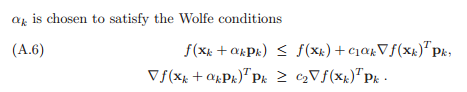

Then the following is the whole L-BFGS algorithm: 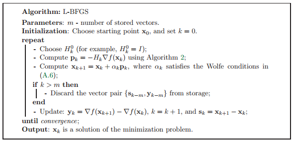L-BFGS

Final Remark Is it really helpful than BFGS?

The following is from the reference OverView of Quasi-Newton Methods:

Note that this process requires only storing $s_i$ and $y_i$ for $𝑖 = 1 … 𝑚,$ or $𝑂(𝑚𝑛)$ floating-point values, which may represent drastic savings over $O(n^2)$ values to store $𝐻$ . After each iteration, we can discard the vectors from iteration $𝑘 − 𝑚$ , and add new vectors for iteration $𝑘$ . Also note that the time required to compute $𝑝$ is only $𝑂(𝑚𝑛)$ .